Conducting a Distance Azimuth Survey

Introduction

Figure 1 - This is a laser distance finder.
There is a second smaller component
not shown here that is placed at the
destination object.  This portion gets
pointed directly at the smaller component
and then the laser reads how far away the
two components are from each other.

     Survey data can be useful for many different applications and there are many different ways that surveys can be done.  Recent technology can allow you to acquire very accurate readings about objects' locations, but they also have their share of problems.  Technology does not always work correctly, therefore it is important to know traditional methods of survey.  For this exercise, the groups were required to use hand instruments to conduct a field survey of a quarter hectare to a hectare area of interest.  The members of our group learned how to you an azimuth compass (Figure 2), a laser distance finder (Figure 2), and a TruPulse Laser (seen in Figure 3) that measures both distance and azimuth during the in class demonstration on February 17, 2014.  To survey our study area, we decided to only use the TruPulse Laser.  We decided to take these points around Governor's Hall on upper campus at the University of Wisconsin-Eau Claire.  We decided to take laser points at three different locations and took data points of trees, snowmen, snow piles, picnic tables, light poles, electrical boxes, doorknobs, frisbee golfing holes and signs, and other various signs.  We conducted our survey on February 21, 2014, which was the day after Eau Claire experienced blizzard like conditions and accumulated an extra 10 inches (minimum) of snow.  Cody is shown below to try to demonstrate how deep the snow was (in Figure 4).  

Figure 2 - This is an azimuth compass.  To give an azimuth reading, hold the device up to your
eye and point it at the destination object.  Keep both eyes open so you can see the object in question.
The compass will show an azimuth reading inside.

Figure 3 - This is the field equipment used to conduct the survey.
The main instrument we used was the TruPuse Laser distance
 finder, which is labelled with "RW" in this photo.

Figure 4 - Here is Cody cold and miserable while demonstrating
 how deep the snow was on the day the survey was conducted.
This provided a good challenge for our survey.

The members of my group were the same as the previous lab: Cody Kroening and Blake Johnson.

Methods

Data Collecting

     Before even going out in to the field, we checked to see what the magnetic declination was for Eau Claire, WI.  Magnetic north is different from true directional north.  The declination is the difference between magnetic north and true north.  This is needed because the devices can have the declination set on them.  Also before going out into the field, we needed to set up a geodatabase for this exercise.  This helps organize the data, especially once tool from ArcToolbox start to be used.

     When thinking about a study area, we were thinking of a place that would have many features that we could take point data on.  We decided to do our survey around Governor's Hall because there are many trees to take point data on (general map shown by Figure 5).  Also, with the influx of snow, there were large snow piles from plowing the roads and sidewalks, and some of the students had also made snowmen and snow forts that could act as points in our survey.

Figure 5- This is a general map of Eau Claire.  The UWEC campus is in the center of this map.  The red star represents a view of where our study area is in context with the city.

 The first location of our survey (represented by the red star in Figure 6) was at the campus side of the fence.  We followed the inside edge of the north wing of the building and walked until we reached the fence.  We figured this would be an easy place to identify on a map because the fence is right at a dramatic tree line.  The second location of our survey (represented by the yellow star in Figure 6) was on the north side of a picnic table and shelter.  We thought this would also be an easily visible feature on a map, but we found this somewhat difficult to find.  The third location of our survey (represented by the blue star in Figure 6) was in front of Governor's Hall.  We stood  right where the ramp ended in front of the main door.

Figure 6 - This is an aerial photograph of our study area.  The three colored stars are our specific positions we were in when acquiring distance and azimuth data.

The TruPulse Laser distance finder was being operated by one group member while another group member recorded the data (Figure 7).  This increased our efficiency and decreased the amount of time we needed to spend outside.

Firgure 7 - One page of data handwritten while in the field.

Importing the Data

     The first step was to find the approximate coordinates of where each of our locations were that we stood.  To do this, we looked at aerial imaging on Bing maps and put our cursor over our locations.  When taking note of these coordinates, we needed to take these numbers out to six decimal places.  This is a formatting issue in ArcMap that the previous class stumbled upon.  We used these coordinates in our Excel table along with other notes we took when we were in the field (Figure 8).  

Figure 8 - This is what our data looks like in Excel.  We made sure to note the feature,
 its azimuth, its distance, and some attribute about the feature.  These types of attributes differ what kind of feature it is.

In order to get the data to display in ArcMap, a few tools needed to be used.  First we used the "Bearing Distance to Line" tool, which is found in the "Data Management Tools" then the "Features" portion of the ArcToolbox (Figure 9).

Figure 9 - This figure is just showing how to navigate to the "Bearing Distance to Line" tool in ArcMap. 

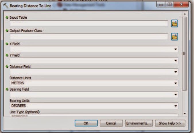Figure 10 - This is the window that pops up when you click on the "Bearing Distance to Line" tool.  The Excel sheet that contains all the data is the input table.  The output feature class needs to be put in the geodatabase that was created earlier.  The X Field and Y Field correspond to the x and y coordinates in the Excel table.  The distance field corresponds to the distance away the features are to the observation point and the bearing field corresponds to the azimuth direction the feature is from the observation point.

Figure 11 - This figure shows how to navigate to the "Feature Vertices to Points" tool in ArcMap.

Figure 12 - This is the box that pops up when you open the "Feature Vertices to Points" tool.  The input features is the new feature class that was created with the "Bearing Distance to Line" tool.  The output will also go in the geodatabase that was created earlier.

Results

     Since we had three different locations that we took data from, we showed them in three different colors to see the data better (Figure 13).  We put imagery as a basemap in ArcMap to show where the data was in relation to real world locations.  Figure 13 is the result of running the "Bearing Distance to Lines" tool and the "Feature Verticies to Points" tool in ArcToolbox on the collected data.
     Most of our data looks like it turned out pretty well.  There are a few lines that do not look accurate because they go through buildings.  We only surveyed features outside, so this should not have appeared in the data.  The imagery available obviously does not include snow, which is a hindrance to see if our points were actually in the right spot all the time.  Some of the features we surveyed were snowmen, snow forts, and snow piles, which we won't be able to tell if they are in the right spot of not.

Figure 13 - This is the resulting map of the three locations we took the survey at.  The red points and lines represent data from the first location, the yellow points and lines represent data from the second location, and the blue points and lines represent data from the third location.

Conclusions

     There were a few points that ended up being mapped in a place that was not their true location.  This could be from our initial observation point that we chose on a map to get the coordinates for our three locations.  We could have been slightly off, getting different coordinates than where we actually were.  The materials that the buildings are made of could have also thrown off the device a little bit.  Since the snow was about 15 inches deep and the blustery conditions, it was difficult to conduct this kind of survey.  If the weather would have been different, I think we could have taken more points and had more attributes for each of the point data.  We could also have spent more time checking the differences between different instruments for collecting the data.  That way we could compare the equipment to see which device was more accurate for the survey.
     The exercise was a useful hands on experience to teach about more traditional methods of surveying.  We did not take any survey stations or even a GPS out to the field with us because we wanted an end product of  a survey using smaller more simple tools.  These methods may take longer to do than a piece of equipment that does it automatically, but now my group members and I are prepared to do a field survey if that equipment fails to work.  We do not have to blindly rely as heavily on our equipment to do the work for us, because we know how to take data with more traditional methods.