Navigation at the Priory - Round Two

Introduction

     Last week at the priory, each group was required to maneuver through the navigation course with only a map and a compass.  On May 5, 2014, each group was required to go through the entire navigation course, but this time we were actually given a GPS unit (reference map in Figure One).  

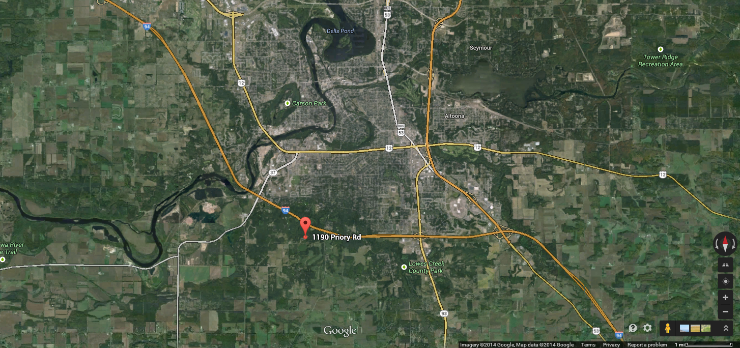
Figure One - The is the general location of the where the priory is.  Interstate 94 and Hwy 53 are shown for reference.

     Before going to the priory grounds, we were required to load one of our maps that was made a few weeks ago in a Trimble Juno with the data of each of the points included in our map (Figure Two).  The process of finding the each checkpoint is made to be more efficient because the GPS tracks exactly where we step.  One added aspect on this exercise is that everyone was armed with a paintball gun!  If any member of your group was shot with a paintball, your whole group had to remain stationary for about one minute, as the goal of this exercise is to be the first one through the whole navigation course.  This made things a little more interesting.

Figure Two - This is the map that our group loaded into our Trimble Juno GPS unit.  There is a colored and transparent DEM on top of imagery that was taken with LiDAR data collection on May 13, 2013.  The yellow points are the navigation points and the red line was the path that our group decided to take.  Contours are labeled in blue.  The areas in pink are "no shooting" zones due to the fact that they are either close to a road or children areas.

Methods

     Every group needed to get through the entire navigation course at the priory, but every group started their navigation at a different checkpoint.  This was done to try to ensure that groups would not run into each other too much.   Our group had to start at the northern most point in the navigation course (marked with a yellow star in Figure Two).  This was somewhat of a disadvantage for our group because I felt like most of the other groups had starting points much closer to where the initial class meeting spot was.  Our group was shot at before we even made it to our starting point.  We used the Trimble GPS to tell us which direction to go for each of the checkpoints.  Our path was being tracked, so it was easy to see if we were going the right direction or not.  While getting from one point to the next, we always had to be aware of our surroundings because you never know who is hiding behind a nearby tree with a paintball gun.  We had to keep our face masks on the whole time just in case someone would sneak up on you.  We were also not allowed to shoot anyone if it looked like they were not wearing a face mask.  

Figure Three - This is what the Trimble Juno GPS units look like.  They have a large touch screen and a built in stylus to assist with operation.

     My role in our group was to be the one manning the GPS unit and figuring our which direction we needed to go to get to our next checkpoint.  Blake was usually the one who went out ahead of us to see if any other group was nearby.  When we would find the checkpoints, I would be the one to take a point in our GPS while Blake scouted the area to make sure we would not get shot at.  Cody would stand right next to me when I would take a point to be my set of eyes on the woods while I was dealing with the GPS unit.  Each role was important and allowed us to be relatively efficient throughout the exercise.  We had a track log running for the entirety of the navigation and took photos of each station just in to prove that we went to each check point if the track log failed to work.

Results

     Our track log was on the whole time and turned out to be quite accurate to what our path actually was.  We turned it on when we were still at the class meeting spot, so our actual starting location of the track log was near the southwest end of the mapping area.  Our group did stick with the path that we had earlier agreed upon, but the track log shows deviations from the straight line segmented path (Figure Four).  

Figure Four - This map shows our planned path in yellow, which was decided before going out into the field based on elevation and distance factors.  The blue dots represent our track log throughout the navigation course.

     Because our team had such great team work, we only got shot once by another group even though we were in quite a few different battles.  We also hit at least two teams along the way.

Discussion

     A few of the deviations in our track log were intentionally done to avoid getting shot by other groups.  This was especially true for the points that are furthest west in the mapping area.  When attempting to get from our third to fourth point, we heard two other groups firing at each other, so we decided to move further west until we heard their battle die down.  This is why there is a bit of a cluster of points on our furthest west points in the track log.  Other deviations were from elevation factors or had to do with getting through the path of least resistance.  With the varying topography, sometimes it is just easier to go down a hill in a way that isn't a straight line from your last point.  Also, since this area was so heavily forested, the abundance of standing trees and trees that were knocked over impeded on our original path.  

Conclusions

     This was a really great exercise for our Geospatial Field Methods class.  We had the luxury of using a GPS to get from one point to another, but had the added "stress" factor that people are wanting to shoot at you.  This forced groups to think on their toes, be aware of their surroundings, and try to be efficient and get through the course as quickly as possible.  Every group was able to navigate through the course with little paint damage to their team.  This proved that each student was able to do field work under pressure, which is helping to prepare us for a professional situation.  Not to say that you will be shot at with a paintball gun in a job setting, but there will always be some pressure to do a job efficiently and accurately.

Navigation at the Priory - Round One

Introduction

     Traditional orienteering skills are important for any person to have.  Technology should never be relied on completely for navigation.  Advances in technology have been extremely helpful in many ways, but it can always fail.  In a previous blog, I talked about how our Geospatial Field Methods class was lucky enough to have an orienteering lesson from Al Wiberg who works at the Environment Adventure Center (EAC) at UW-Eau Claire.  Now we got to apply these skills in the field!  There is an orienteering course that is located in the woods around the priory (Figure One).  Maps of the priory were also created in previous exercises and printed out for this lab.  Our class carried out this navigation exercise on Monday, April 28, 2014.  As long as you have a map and a compass, navigation is possible.

Figure One - This is the general location of where the priory is.  Interstate 94 and Hwy 53 are shown for reference.

Methods

     When arriving at the Priory, each group was given a list of all the points and their corresponding coordinates given in both UTM and decimal degrees.  Each team had two priory maps that were made in a previous exercise: one with a UTM coordinate system grid, and the other with a decimal degree grid.  We were required to plot our teams given navigation points on our maps using whichever map we felt more comfortable with.  Personally, I am used to using the UTM grid system, so I plotted our points on our UTM map (Figure Two).

Figure Two - This is my map board with with my field book and punch card on the left and the priory map on the right side.

About two teams of students were given the same third of the course to navigate, so all the teams would not run into each other or navigate through the course together.  To get form one point to another, a straight-edge was used to line up where we were with where we wanted to get to.  An azimuth was taken on that line in relation to where we were.  Three people were on our team and each person had a particular job as we navigated through the course.  I found the azimuth of the point we needed to get to next based on where we currently were, as well as being the pacer.  Blake was the one with the compass and stood stationary while he directed the "runner" where to go to follow that given azimuth.  Cody was our "runner" and acted as a trailblazer for Blake and I.  Blake would tell Cody which direction to go by giving him checkpoints (Figure Three) and Cody would make his way to that checkpoint.

Figure Three - Blake is directing Cody in the correct direction based on the azimuth we were trying to follow.

I would start at Blake's position and walk towards Cody's checkpoint in as straight of a line as possible.  As I did so, I counted the steps it took to get there.   This helped us gauge how far we had gone from the previous point and how much further we needed to go in order to make it to your next check point.  In a previous lab for Geog 336, every student figured out their pace count for navigation exercises like this.  My pace count was 68 steps equals about 100 meters.  Each checkpoint had a small orange tent like object so it could be seen more easily in the forest (Figure Three).

Figure Three - This is what each checkpoint of the navigation course looked like.

At each checkpoint, we had to use the orange clamp that hangs from the tent on a string, on our punch cards at the appropriate spot.  During this exercise, each group only had to navigate through five points of the course.

Results

     Our team made it out alive (Figure Five)!  And we had about a half hour of time to spare.  

Figure Five - Here stands Cody and Blake with a completed punch card for our part of the navigation course.

Discussion

     Our group had great team work, which allowed us to successfully navigate through the course at the priory.  We got flustered a few times when we could not find the checkpoints right away.  This is where it would have been helpful to have a GPS unit to gauge where we are in terms of the desired checkpoint.  We got especially flustered when one of the checkpoints was not where we thought it was, but this problem could stem from many aspects of the exercise.  When we plotted the points on our map before beginning the navigation course, it is possible that the points were not placed in exactly the right spot.  Each point had very accurate coordinates, but we were just drawing the points on a paper map, which cannot get nearly show that accuracy.  Also, when doing a pace count in an area, it is easy to have consistent steps when walking on a flat surface.  This exercise was mostly in a wooded area with some topographic changes.  Maneuvering uphill, downhill, around objects, and over fallen trees means that each step will not cover the same distance as a normal step.

Conclusion

     Despite the fact that we did not find all the points right away on the first try, I think all of our group member learned valuable lessons on this day.  We were able to navigate around in a mostly wooded area without a GPS unit, with only a compass and a map to guide us.  We worked together, even when we ran into problems.  Team work is definitely essential in an exercise like this.  Everyone needs to be open to the other group member's thoughts and opinions about how to become more efficient.  It is interesting to think that it took each group almost the full three hours to complete only a third of the navigation course.  Next time we come to the priory, each group is required to complete the entire navigation course, but we will have a GPS unit next time.  Hopefully we can finish the whole course in the allotted three hours!

UAS III - Balloon Mapping

Introduction

     Unmanned aerial systems (UAS) can take on many different forms.  In previous labs we learned how basic UAS units work and the different ways to attach a GPS and a camera.  On Monday, April 21, 2014 the Geog 336 class returned to the Eau Claire Indoor Sports Center grounds (Figure One).  The plan was to get really good imagery of the entire property and a little outside of it.  This required group thinking in how we would make sure to cover the whole are and get enough overlap to make sure not spots were skipped over.

Figure One - At the center of this map is the Eau Claire Indoor Sports Center grounds.

Methods

Balloon March

     A large weather balloon was used as our UAS for the day.  In order to fly the balloon, it needed to be filled up with helium.  When properly filled up, the balloon was about three feet in diameter (Figure Two).

Figure Two - Cody is holding on to the balloon to that it does not fly away before we are ready.

After completely filled, a hardy piece of rope on a spool was attached to the balloon so we could have control over it.  An additional string attached to the rope holds the GPS and the camera (Figure Three). 

Figure Three - Joe Hupy has just attached a simple camera and GPS to the balloon rope by a string.  The weight of the devices should be enough to keep the camera point downward.

The camera was set to take a photo every five seconds.  About four students traded off having control of the balloon while the camera was snapping photos.  

PhotoScan

Click Workflow on the Tab list.  Click Add Photos.  Only add the photos that are necessary.  If many (over 200) pictures are used, the program will take hours to complete the process.

When the photos are added, return to the Workflow tab and click Align Photos.  This will create a point cloud.  Click Build Mesh to create a Triangulated Irregular Network (TIN) from the point cloud.

Next, click on Create The Texture under the Workflow tab.  This needs to be turned on in order to see a difference in your images.  Look for the Texture icon under Tabs to do this.  Cameraicon can be clicked to turn off the blue squares.

To able to use the image in other programs, it needs to exported as a .jpg, .tiff, or a .png file format (Export Orthophoto).  A .tiff files may be best.  This file can now be brought into ArcMap.  It would also be a good idea to add imagery as a basemap.

Open the Geoprocessing Tool-set in ArcMap and click on the Viewer icon (button with magnifying glass).  The .tiff file will open in a separate viewer.

Control points need to be added to the photo shows up where it is supposed to be spatially (Add Control Points).  Once this option is clicked, select a point on the orthophoto, then click on corresponding location on the satellite image.  Get a widely dispersed set of control points to pin down the orthophoto against the ArcMap basemap.  At least 10 control points should be used to ensure that the photo is not skewed, stretched, or otherwise distorted in any way.  Once this is done, click Rectify in the Georeferencing toolbar.

Geosetter 

In Geosetter, the images that you want to use need to be selected.  They will go into a separate viewer box.  Make sure none of the photos have blue markers on them, this mean coordinates are attached to them.  

Click on the icon labeled "2" in Figure Four.  This makes the tracklog embed and select-able into the images.

Click Synchronize with Data File in the new window that opens up.  Input the GSX track log (Figure Five).

Figure Four - The GeoSetter interface.

Figure Five - Embedding the tracklog by time into the images.

To save images, close the program and click "yes" when the prompt asks you to save.  The coordinates will also be saved to the images.

Results

Figure Six - This image shows the amount of overlap of the images used in the mosaicking process.

Figure Seven - This is the result of the mosaicked images.  The orientation is not corrected because it has not been georeferenced yet at this stage.

Figure Eight - This is the result of the images from the other camera.  This camera took images that were a little darker, which can easily be corrected, but this is the raw data.

Figure Nine - This is a DEM of the mosaicked georeferenced orthophoto.  

Conclusion

     Using a balloon for a UAS was found to actually work pretty well.  Even with a cheaper digital camera and GPS, mapping from imagery can still be done.  The combination of these collection methods along with PhotoScan and GeoSetter can make a fairly accurate map even on a budget.  Planning is still an essential part of flying this kind of UAS.  If the weather would have been poor that day, the balloon may have not been the best choice for a UAS.  Luckily, the day our class went mapping was relatively sunny and the wind was not too bad.  If time was an issue, the balloon may not be the best choice either.  Walking with a balloon on a rope can be time consuming, especially if the area of interest is larger.  For the purposes of this exercise, the balloon mapping worked very well.

UAS II - Mission Planning

Introduction

     Advances in technology have allowed for people to significantly increase the amount of data and its accuracy.  This is especially true with the growing use of unmanned aerial systems (UAS).  There are many things to consider prior to field work and during field work that will help and UAS study successful.  The work that is done before going out into the field is called "mission planning" as you need to know ahead of time all aspects of your area of interest and how your equipment will effectively cover the entire area.  Knowing your equipment inside and out is essential in conducting a study with a UAS.  The Geog 336 class went to the Eau Claire Indoor Sports Center grounds (Figure One) on Monday, April 14, 2014 to learn about UAS mission planning.  We use a three armed, six propeller fixed wing aircraft can travel at about 5 meters per second (Figure Two).

Figure One - At the center of this map is the grounds for the Eau Claire Indoor Sports Center.

Figure Two - Joe Hupy's fixed winged UAS that can travel at about 5 meters per second.  The unit has a typical battery life of about 15 minutes.  A simple Canon digital camera is attached to the bottom of the unit which is set to swivel so it is always pointing downward.

Planning Methods

     Before flying a UAS in the field, it is important to remember a couple things.  First of all, it is very important to make sure that the batteries are fully charged and that the transmission is working.  The weather should be checked before a UAS flight.  Obviously if it is raining, you may want to consider changing the flight day so to avoid damage to any of your equipment.  Also, it is important to note that if it is a particularly cold or windy day, this will drain the batteries faster on the UAS.  Understanding the topography and foreign objects (such as buildings) in your mapping area is essential.  If either of these factors are at a high enough elevation, it may be possible that the UAS would collide with them.  The user needs to plan to fly above or around these objects.  Elevation data (z-coordinate) is not very very good with many GPS units, but a good average altitude to fly a UAS at is about 100 feet.  Since z-coordinates are not high in accuracy, it would be a good idea to give yourself enough of a buffer to go around objects that have a relatively high elevation.  The user can decide if they want the UAS to loiter within that polygon or if they want the UAS to visit certain points during its flight.  A survey grid or footprint should be used to make sure there is a correct amount of overlap across imagery scans.  

Figure Three - Joe Hupy watches the software as
the UAS is in flight to make sure all the vitals of
the equipment is in check. 

     A checklist should always be made for a UAS flight.  The UAS will land wherever you tell it to land, despite what objects may be in that spot when the UAS is supposed to land. The user can set up the UAS so that it returns to the same place it took off from.  The whole process should not be done by one person alone.  One person should be at the computer the whole time watching the battery life and making sure the UAS stays on the proper course (Figure Three).  One person should be the commander pilot that knows how to fly the UAS manually, for those "just in case" scenarios.  One person should be the engineer that is able to deal with any software issues if they were to occur.  The one manning the computer should make sure that auto pilot is working at all times during the flight (green light).  When the battery power is at about 60%, it is a good idea to start bringing the UAS to its landing point.  The flight will have to be interrupted and the UAS will have to be commanded to forget about the remainder of the mission and go directly to the landing point.  Something to keep in mind when the user goes to retrieve the UAS is that the engine should be turned off before picking it up.

     Free software is available for download for unmanned aerial system flights.  Within this program, a polygon can be drawn around the area of interest and weigh points can be added depending on where the user wants the UAS to travel to.  An exact flight plan can be executed, or the UAS can be set to loiter within that polygon that was drawn around the area of interest (Figure Four).  The software for these kinds of applications are being updated fairly often, so it is uncommon for manuals to be written for this kind of program.  Discussion forums and blogs are the more common way to communicate comments and issues about software packages.

Figure Four - This shows a quick look at what the planned flight path of the UAS was in the software program.  The green dots represent the weigh points the UAS is set to go to and the yellow line is the planned flight path of the UAS.

Results

     Figures Five through Eight are a few images that were collected during the UAS flight conducted by Joe Hupy.  The images turned out to be a little dark because the weather was slightly overcast that day.  Images could be brightened up with Photoshop, but I wanted to show what the raw data looked like that was collected from the Canon camera that was attached to the bottom of the UAS.

Figure Five - Image over a neighborhood house nearby the Eau Claire Indoor Sports Center grounds.

Figure Six - An image of a road near the Eau Claire Indoor Sports Center.  It is apparent just from doing a short exercise like this that the roads in the area are in less than perfect shape.  This could be one of many applications of these methods.

Figure Seven - This is an image the UAS took while it was returning to its launch site after flying over a nearby neighborhood.  This photo must have been captured right when the UAS changed direction, because the camera did not get a chance to point itself downward.  

Figure Eight - This is a photo of the top of the main pavilion of the Eau Claire Sports Center.  This is towards the end of the UAS flight as the unit is returning to its launch location.

Conclusion

     Advances in unmanned aerial systems have made imagery applications much easier and more efficient.  Mission planning of the flight of a UAS is almost more important that knowing how the unit flies.  There are so many factors that could make a flight fail, that it is important to consider all the possibilities before even beginning a flight.  The more knowledge and experience the user has, the more effective and efficient a UAS flight can be.

Topcon Total Survey Station

Introduction

     In this Geospatial Field Methods course, we have learned a variety of surveying techniques that require very minimal equipment.  In this exercise, we used a high end piece of equipment to survey the campus mall area at the University of Wisconsin-Eau Claire.  The Topcon Total Survey Station along side the GMS-2 handheld GPS system gives a much higher accuracy of X, Y, and Z coordinates.  With previous methods of surveying, elevation values (Z coordinates) could not be acquired.  We spent one entire class period learning how to set up the Topcon Total Survey Station in the classroom setting.  This is a very expensive piece of equipment, so we were all required to know the steps in just setting up the station before actually putting it into use.  Even with preparation, groups ran into a few issues when executing this survey activity.

Methods

     Setting up the Topcon Total Survey Station properly is almost more important than performing the survey.  The tripod that the Topcon sits on top of has three legs that need to be spread wide enough that the whole device will not tip over (Figure One).  Once the legs of the tripod are evenly spaced, one person should step on the small ledge near the bottom of each leg and push it down into the ground to ensure stability of the station.  The tripod should also be made as level as possible before even attaching the Topcon to it.  This can be done by adjusting each of the telescoping legs of the tripod.  Now the Topcon can be attached to the top of the tripod.  A piece on the bottom of the Topcon needs to be unscrewed before placing it on top of the tripod.  This piece gets screwed back on the bottom of the Topcon, but this time through the tripod.  This ensures that the Topcon will stay atop the tripod while conducting the surveying exercise.  There are a few levelers on the Topcon that assist in making the system completely horizontal.  The telescoping legs should be adjusted on the tripod as needed to get the Topcon level.  Additional air bubble levelers should viewed while turning the four round black nobs that the Topcon sits on, to get the system more precisely level.  The height from the ground up to the lens of the Total Station should be noted as it will need to be put into the GMS-2.
    

Figure One - Drew and Tanner are setting up the base for the Topcon Total Survey Station during the class's initial day learning how to set up the equipment.

   
     Once the Topcon Total Station is set up and leveled, the cover must be taken off of the front lens and the system can be powered on with the green power button on the system.  The tilt should be checked to make sure the whole station is not too far away from being level.  The laser plummet should also be used to check if the center of the station is over the point that you want it to be.  This is denoted with a star on the Total Station.  If the station is centered over the desired point, then the blutooth needs to be turned on with the Total Station (Menu--> F4 --> F4 --> F2 --> F4 --> F4 --> F3 --> "Enter" to set).  Using the handheld GMS-2 device (Figure Two) now, the project needs to be selected.  The software program used for this is called "Topsurv" and it should recognize the blutooth of the Total Station.  Then the occupied point and the backsite need to be set up on the Total Station.  In the "collect" menu, chose "OCC/BS setup."  Have one person in your group stand at a location and shoot it with the Total Station.  Use a conventional compass to find the azimuth of that point and record that in the handheld GMS-2 device.  Do the same for the backsite.  This is the step that will ask for the height of the Total Station as well as the height for the reflector.  For our survey,  the azimuth for our backsite was 322,º the height of the Total Station was 1.52 meters, and the height for the reflector was 2 meters. 

Figure Two - A look at the GMS-2 handheld
piece of equipment that goes along with the
Topcon Total Survey Station.

     Now the data collecting can begin!  In the main menu of the Topsurv software, go to collect, then select topo, then measure.  One person in the group needs to stand at the survey point with the reflector that is on a pole at a fixed height throughout the survey (Figure Three).  Another person needs to peer through the Total Stations scope towards the reflector.  Once they have it sited, the third person clicks collect on the GMS-2 (Figure Four).  The Total Station recognizes the azimuth and the elevation of the location of the reflector relative to itself based on information from the set occupied point.  Our surveying group took 116 points and tried to take them in a somewhat systematic way.  We started on the west side of our mapping area and tried to make 8 step intervals between each collection point.  Each row of data we collected trending north-south, and each row was progressed west to east.  By having this methodology in collecting the data, I believe we got a decent coverage of the area of interest.

Figure Three - Nate is poses with the reflector, showing that you
need to stand perfectly still in order for the person manning the
Total Station to shoot it with a laser.

Figure Four - Blake operates where the measurement
is going to be taken with the Total Station while I operate the GMS-2.

     Once all the data points were collected, they needed to be exported from the the GMS-2 to a computer.  To do this, go to the "Export" menu and chose "To File."  The data can be exported as a .txt and a .shp, but the projection and the datum need to be the same as what the data was collected in.  Also, the delimiter needs to be set to comma.  The data was able to be opened in Notepad and then exported as a table that could be opened up in Excel.  We did this just to make sure the data was exported in the correct format.  From here, the table can be added to ArcMap and the X and Y data can be displayed with the elevation data attached to it.  To interpolate what the elevation would be in the area between the points, a kriging method was used.  This creates a continuous surface with a pretty good idea of what the elevation is across the area of interest.

     

Results

     Our group took 116 points across the new campus mall area (Map shown in Figure Five).  We realized that some of our points are more bunched together than other points.  If we would have exactly measured out where each point was going to be, our points may have been more evenly distributed.  This may have also been the case because each group member switched roles throughout the survey, so that everyone would get hands on experience with all pieces of the equipment.  This means that different people were pacing out the distance between each point during the survey.  For example, Blake is taller than I am, so he is likely to have bigger strides than when I was holding the reflector.  Having said that, our methodology worked well for getting a relatively quick survey of an area.  

Figure Five - This is resulting map of our surveying using the Topcon Total Survey Station.  Each individual survey point is shown as well as the relative elevation based on the interpolation method of kriging.  The elevation change is not very great across our area of interest, so the color spectrum from the interpolation may make the elevation differences seem larger.  The background image was collected when LiDAR data was collected from May 13, 2013.  

     

     

Discussion

     While executing this survey, our group encountered a multitude of problems.  When we were setting up our occupied point, the "HTC Set" button would not click on our handheld unit.  After many attempts of clicking, the system would tell us that the bluetooth needed to be reconnected.  This happened many times while this "HTC Set" would not click.  Somewhere within this process, the Topcon Total Station shut down and we had to reboot it.  When the system rebooted, the handheld unit then allowed us to click the "HTC Set" without being interrupted by a bluetooth warning.  After the whole system rebooted, the bluetooth warning did not return for the rest of the exercise.
     When looking to start collecting points, our group had a hard time finding which menu to go into to actually collect the points.  The directions only said to go to "col" menu and go into the observations tab, but what we really had to do was go into "topo" menu and from there navigate to the "measurement" option.  From there on out, our data collection seemed to go smooth.
     Exporting the data we collected in the field also had an unexpected snag.  We exported the data from the GMS-2 as a text file (.txt) and as a shapefile (.shp).  When opening either file type in their appropriate programs, only the occupied point showed up.  The GMS-2 system appeared to have been collecting data, but that data was not exporting into the data files.  I believe this might have something to do with when the Topcon Total Station rebooted itself when we were attempting to set our occupied point.  The GISP at UW-Eau Claire, Martin Goettl, was nice enough to recompute our data to show up.

Conclusions

     Getting hands on experience with the Topcon Total Survey Station was a very useful exercise.  Using any sort of equipment for the first time will always have its problems and downfalls.  I only wish there was more time to maybe take the equipment out to another location and survey areas outside of our UW-Eau Claire campus.  I think it was a good idea for us to learn how to set up the Total Station before going out to collect the data.  This probably eliminated a lot of the errors that could have been present.  This surveying process definitely requires at least two people, but having three people per team allowed each member to really focus in on their specific task.  Conventional survey methods are great to know, but using this kind of equipment to conduct a survey allows for much more accurate data, which is always a plus.