May 13, 2014

UAS II - Mission Planning

Introduction

     Advances in technology have allowed for people to significantly increase the amount of data and its accuracy.  This is especially true with the growing use of unmanned aerial systems (UAS).  There are many things to consider prior to field work and during field work that will help and UAS study successful.  The work that is done before going out into the field is called "mission planning" as you need to know ahead of time all aspects of your area of interest and how your equipment will effectively cover the entire area.  Knowing your equipment inside and out is essential in conducting a study with a UAS.  The Geog 336 class went to the Eau Claire Indoor Sports Center grounds (Figure One) on Monday, April 14, 2014 to learn about UAS mission planning.  We use a three armed, six propeller fixed wing aircraft can travel at about 5 meters per second (Figure Two).

Figure One - At the center of this map is the grounds for the Eau Claire Indoor Sports Center.

Figure Two - Joe Hupy's fixed winged UAS that can travel at about 5 meters per second.  The unit has a typical battery life of about 15 minutes.  A simple Canon digital camera is attached to the bottom of the unit which is set to swivel so it is always pointing downward.


Planning Methods

     Before flying a UAS in the field, it is important to remember a couple things.  First of all, it is very important to make sure that the batteries are fully charged and that the transmission is working.  The weather should be checked before a UAS flight.  Obviously if it is raining, you may want to consider changing the flight day so to avoid damage to any of your equipment.  Also, it is important to note that if it is a particularly cold or windy day, this will drain the batteries faster on the UAS.  Understanding the topography and foreign objects (such as buildings) in your mapping area is essential.  If either of these factors are at a high enough elevation, it may be possible that the UAS would collide with them.  The user needs to plan to fly above or around these objects.  Elevation data (z-coordinate) is not very very good with many GPS units, but a good average altitude to fly a UAS at is about 100 feet.  Since z-coordinates are not high in accuracy, it would be a good idea to give yourself enough of a buffer to go around objects that have a relatively high elevation.  The user can decide if they want the UAS to loiter within that polygon or if they want the UAS to visit certain points during its flight.  A survey grid or footprint should be used to make sure there is a correct amount of overlap across imagery scans.  
Figure Three - Joe Hupy watches the software as
the UAS is in flight to make sure all the vitals of
the equipment is in check. 
     A checklist should always be made for a UAS flight.  The UAS will land wherever you tell it to land, despite what objects may be in that spot when the UAS is supposed to land. The user can set up the UAS so that it returns to the same place it took off from.  The whole process should not be done by one person alone.  One person should be at the computer the whole time watching the battery life and making sure the UAS stays on the proper course (Figure Three).  One person should be the commander pilot that knows how to fly the UAS manually, for those "just in case" scenarios.  One person should be the engineer that is able to deal with any software issues if they were to occur.  The one manning the computer should make sure that auto pilot is working at all times during the flight (green light).  When the battery power is at about 60%, it is a good idea to start bringing the UAS to its landing point.  The flight will have to be interrupted and the UAS will have to be commanded to forget about the remainder of the mission and go directly to the landing point.  Something to keep in mind when the user goes to retrieve the UAS is that the engine should be turned off before picking it up.
     Free software is available for download for unmanned aerial system flights.  Within this program, a polygon can be drawn around the area of interest and weigh points can be added depending on where the user wants the UAS to travel to.  An exact flight plan can be executed, or the UAS can be set to loiter within that polygon that was drawn around the area of interest (Figure Four).  The software for these kinds of applications are being updated fairly often, so it is uncommon for manuals to be written for this kind of program.  Discussion forums and blogs are the more common way to communicate comments and issues about software packages.


Figure Four - This shows a quick look at what the planned flight path of the UAS was in the software program.  The green dots represent the weigh points the UAS is set to go to and the yellow line is the planned flight path of the UAS.

Results

     Figures Five through Eight are a few images that were collected during the UAS flight conducted by Joe Hupy.  The images turned out to be a little dark because the weather was slightly overcast that day.  Images could be brightened up with Photoshop, but I wanted to show what the raw data looked like that was collected from the Canon camera that was attached to the bottom of the UAS.
Figure Five - Image over a neighborhood house nearby the Eau Claire Indoor Sports Center grounds.

Figure Six - An image of a road near the Eau Claire Indoor Sports Center.  It is apparent just from doing a short exercise like this that the roads in the area are in less than perfect shape.  This could be one of many applications of these methods.

Figure Seven - This is an image the UAS took while it was returning to its launch site after flying over a nearby neighborhood.  This photo must have been captured right when the UAS changed direction, because the camera did not get a chance to point itself downward.  

Figure Eight - This is a photo of the top of the main pavilion of the Eau Claire Sports Center.  This is towards the end of the UAS flight as the unit is returning to its launch location.

Conclusion

     Advances in unmanned aerial systems have made imagery applications much easier and more efficient.  Mission planning of the flight of a UAS is almost more important that knowing how the unit flies.  There are so many factors that could make a flight fail, that it is important to consider all the possibilities before even beginning a flight.  The more knowledge and experience the user has, the more effective and efficient a UAS flight can be.

May 12, 2014

Topcon Total Survey Station

Introduction

     In this Geospatial Field Methods course, we have learned a variety of surveying techniques that require very minimal equipment.  In this exercise, we used a high end piece of equipment to survey the campus mall area at the University of Wisconsin-Eau Claire.  The Topcon Total Survey Station along side the GMS-2 handheld GPS system gives a much higher accuracy of X, Y, and Z coordinates.  With previous methods of surveying, elevation values (Z coordinates) could not be acquired.  We spent one entire class period learning how to set up the Topcon Total Survey Station in the classroom setting.  This is a very expensive piece of equipment, so we were all required to know the steps in just setting up the station before actually putting it into use.  Even with preparation, groups ran into a few issues when executing this survey activity.

Methods

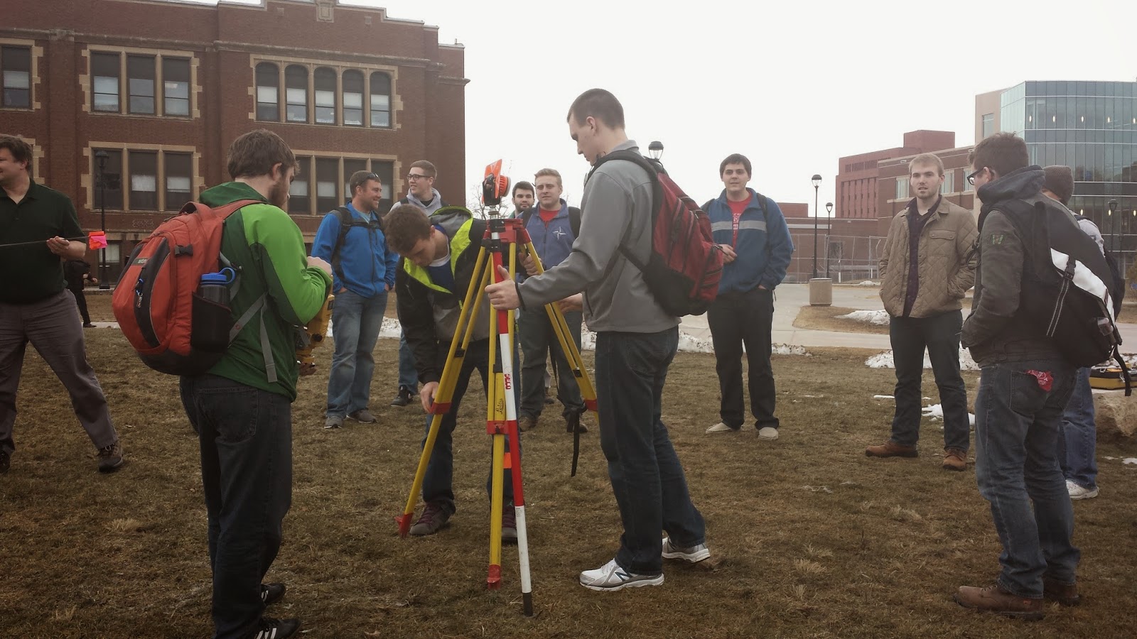
     Setting up the Topcon Total Survey Station properly is almost more important than performing the survey.  The tripod that the Topcon sits on top of has three legs that need to be spread wide enough that the whole device will not tip over (Figure One).  Once the legs of the tripod are evenly spaced, one person should step on the small ledge near the bottom of each leg and push it down into the ground to ensure stability of the station.  The tripod should also be made as level as possible before even attaching the Topcon to it.  This can be done by adjusting each of the telescoping legs of the tripod.  Now the Topcon can be attached to the top of the tripod.  A piece on the bottom of the Topcon needs to be unscrewed before placing it on top of the tripod.  This piece gets screwed back on the bottom of the Topcon, but this time through the tripod.  This ensures that the Topcon will stay atop the tripod while conducting the surveying exercise.  There are a few levelers on the Topcon that assist in making the system completely horizontal.  The telescoping legs should be adjusted on the tripod as needed to get the Topcon level.  Additional air bubble levelers should viewed while turning the four round black nobs that the Topcon sits on, to get the system more precisely level.  The height from the ground up to the lens of the Total Station should be noted as it will need to be put into the GMS-2.
    
Figure One - Drew and Tanner are setting up the base for the Topcon Total Survey Station during the class's initial day learning how to set up the equipment.
   
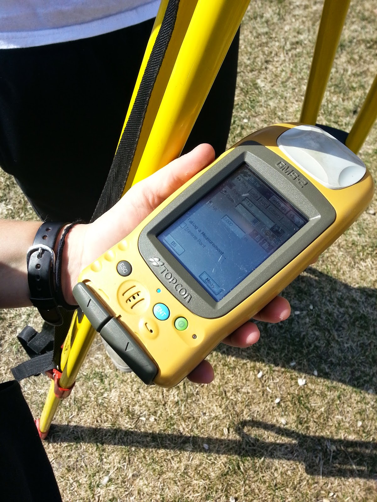
     Once the Topcon Total Station is set up and leveled, the cover must be taken off of the front lens and the system can be powered on with the green power button on the system.  The tilt should be checked to make sure the whole station is not too far away from being level.  The laser plummet should also be used to check if the center of the station is over the point that you want it to be.  This is denoted with a star on the Total Station.  If the station is centered over the desired point, then the blutooth needs to be turned on with the Total Station (Menu--> F4 --> F4 --> F2 --> F4 --> F4 --> F3 --> "Enter" to set).  Using the handheld GMS-2 device (Figure Two) now, the project needs to be selected.  The software program used for this is called "Topsurv" and it should recognize the blutooth of the Total Station.  Then the occupied point and the backsite need to be set up on the Total Station.  In the "collect" menu, chose "OCC/BS setup."  Have one person in your group stand at a location and shoot it with the Total Station.  Use a conventional compass to find the azimuth of that point and record that in the handheld GMS-2 device.  Do the same for the backsite.  This is the step that will ask for the height of the Total Station as well as the height for the reflector.  For our survey,  the azimuth for our backsite was 322,ยบ the height of the Total Station was 1.52 meters, and the height for the reflector was 2 meters. 
Figure Two - A look at the GMS-2 handheld
piece of equipment that goes along with the
Topcon Total Survey Station.

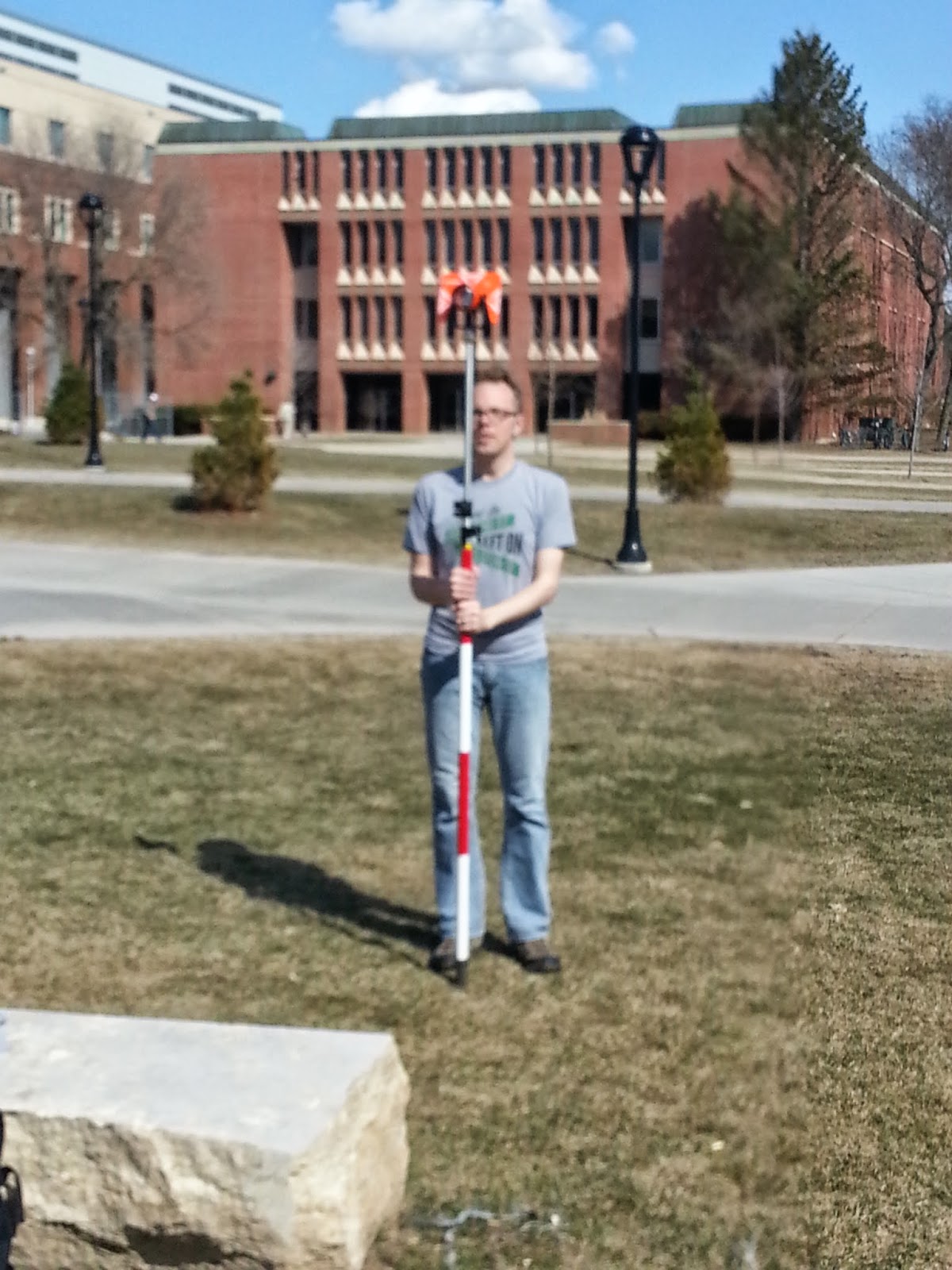
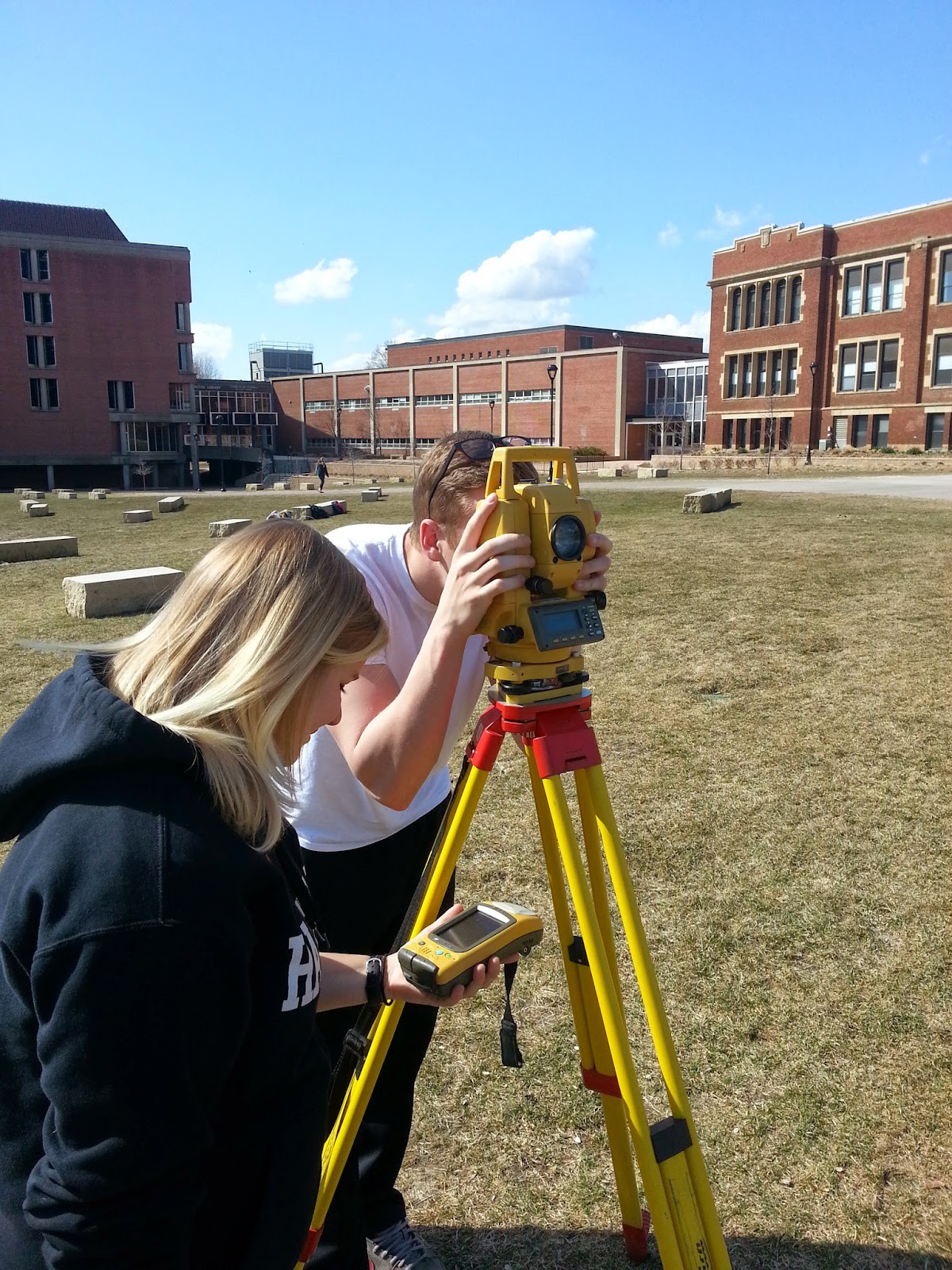
     Now the data collecting can begin!  In the main menu of the Topsurv software, go to collect, then select topo, then measure.  One person in the group needs to stand at the survey point with the reflector that is on a pole at a fixed height throughout the survey (Figure Three).  Another person needs to peer through the Total Stations scope towards the reflector.  Once they have it sited, the third person clicks collect on the GMS-2 (Figure Four).  The Total Station recognizes the azimuth and the elevation of the location of the reflector relative to itself based on information from the set occupied point.  Our surveying group took 116 points and tried to take them in a somewhat systematic way.  We started on the west side of our mapping area and tried to make 8 step intervals between each collection point.  Each row of data we collected trending north-south, and each row was progressed west to east.  By having this methodology in collecting the data, I believe we got a decent coverage of the area of interest.

Figure Three - Nate is poses with the reflector, showing that you
need to stand perfectly still in order for the person manning the
Total Station to shoot it with a laser.
Figure Four - Blake operates where the measurement
is going to be taken with the Total Station while I operate the GMS-2.

     Once all the data points were collected, they needed to be exported from the the GMS-2 to a computer.  To do this, go to the "Export" menu and chose "To File."  The data can be exported as a .txt and a .shp, but the projection and the datum need to be the same as what the data was collected in.  Also, the delimiter needs to be set to comma.  The data was able to be opened in Notepad and then exported as a table that could be opened up in Excel.  We did this just to make sure the data was exported in the correct format.  From here, the table can be added to ArcMap and the X and Y data can be displayed with the elevation data attached to it.  To interpolate what the elevation would be in the area between the points, a kriging method was used.  This creates a continuous surface with a pretty good idea of what the elevation is across the area of interest.
     

Results

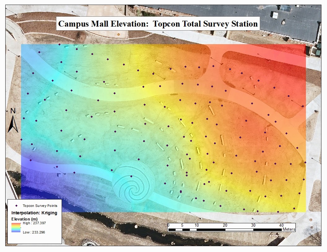
     Our group took 116 points across the new campus mall area (Map shown in Figure Five).  We realized that some of our points are more bunched together than other points.  If we would have exactly measured out where each point was going to be, our points may have been more evenly distributed.  This may have also been the case because each group member switched roles throughout the survey, so that everyone would get hands on experience with all pieces of the equipment.  This means that different people were pacing out the distance between each point during the survey.  For example, Blake is taller than I am, so he is likely to have bigger strides than when I was holding the reflector.  Having said that, our methodology worked well for getting a relatively quick survey of an area.  

Figure Five - This is resulting map of our surveying using the Topcon Total Survey Station.  Each individual survey point is shown as well as the relative elevation based on the interpolation method of kriging.  The elevation change is not very great across our area of interest, so the color spectrum from the interpolation may make the elevation differences seem larger.  The background image was collected when LiDAR data was collected from May 13, 2013.  


Discussion

     While executing this survey, our group encountered a multitude of problems.  When we were setting up our occupied point, the "HTC Set" button would not click on our handheld unit.  After many attempts of clicking, the system would tell us that the bluetooth needed to be reconnected.  This happened many times while this "HTC Set" would not click.  Somewhere within this process, the Topcon Total Station shut down and we had to reboot it.  When the system rebooted, the handheld unit then allowed us to click the "HTC Set" without being interrupted by a bluetooth warning.  After the whole system rebooted, the bluetooth warning did not return for the rest of the exercise.
     When looking to start collecting points, our group had a hard time finding which menu to go into to actually collect the points.  The directions only said to go to "col" menu and go into the observations tab, but what we really had to do was go into "topo" menu and from there navigate to the "measurement" option.  From there on out, our data collection seemed to go smooth.
     Exporting the data we collected in the field also had an unexpected snag.  We exported the data from the GMS-2 as a text file (.txt) and as a shapefile (.shp).  When opening either file type in their appropriate programs, only the occupied point showed up.  The GMS-2 system appeared to have been collecting data, but that data was not exporting into the data files.  I believe this might have something to do with when the Topcon Total Station rebooted itself when we were attempting to set our occupied point.  The GISP at UW-Eau Claire, Martin Goettl, was nice enough to recompute our data to show up.

Conclusions

     Getting hands on experience with the Topcon Total Survey Station was a very useful exercise.  Using any sort of equipment for the first time will always have its problems and downfalls.  I only wish there was more time to maybe take the equipment out to another location and survey areas outside of our UW-Eau Claire campus.  I think it was a good idea for us to learn how to set up the Total Station before going out to collect the data.  This probably eliminated a lot of the errors that could have been present.  This surveying process definitely requires at least two people, but having three people per team allowed each member to really focus in on their specific task.  Conventional survey methods are great to know, but using this kind of equipment to conduct a survey allows for much more accurate data, which is always a plus.

Mar 13, 2014

Introduction to Unmanned Aerial Systems

Introduction

     On Monday March 10, 2014, our Geography 336 class met at the ground of the Eau Claire Indoor Sports Center (Figure One shows a reference map).  There was still a lot of snow on the ground, but the high temperature for the day was 50°F and the sun was shining brightly.  This day was used to get familiar with the different kinds of unmanned aerial systems and the kinds of cameras that can be used to take quick aerial imagery of a small area of interest.  There was a light constant amount of wind, making it not too difficult for the rotary crafts to be flown, but enough to fly the kite successfully.

Figure One - At the center of the map is the Eau Claire Indoor Sports Center

UAV Equipment

Multi-Armed Rotary Crafts

     The first UAV (Figures Two and Three) that we looked at was Joe Hupy's three armed rotary craft.  Each arm had two propellers on the ends of it.  Underneath the main craft was where the camera was mounted.  It was just a normal digital camera that was set to take pictures for a specific interval of time.  It was mounted in a way that no matter which way the aircraft was tilted while flying through the air, the camera was always pointing down.  Joe had a system put in place with his UAV so that you could look through this binocular head set that should exactly what the camera was shooting (Figure Three).  There were settings you could change about the camera right on the head set too.  This craft has a flight time of about 15 minutes.
Figure Two - Joe Hupy's three armed rotary craft in flight.

Figure Three - Nathan is looking through the headset to see exactly what the camera sees.

     Max (shown in Figure Four) is a physics student who has been working with Joe on these unmanned aerial systems.  He basically built this six armed rotary craft as a project (Figures Four and Five).  It only had one propeller on each arm, but having six arms appeared to be a more precise flyer.  Average flight time for this craft was also about 15 minutes.  Max told us that if for some reason something went wrong with the remote control and he wasn't able to drive it himself, the craft was programmed to automatically land at the same location that it took off from.  Technology is amazing!
Figure Four - Max, the physics student, flying his six armed rotary craft over the snow.

Figure Five - A close up of the six armed rotary craft in flight.

     Max flew both of these crafts (Figure Six) successfully just from a little remote control.  He began each flight at a distance away from the group of students just in case the take off was rough or if he would have a difficult time trying to control the craft.  Each craft was landed successfully around the same location without any crashes.
Figure Six - This shows both three and six armed rotary crafts side by side.

Kite

     The next piece of equipment we got to witness was the kite.  The kite was an up scale, but simple kite purchased at a place like Wal-Mart for about $80.  It came with poles that needed to be put together then attached to the kite.  Blake had used this kite in a class field trip to France, so he was appointed to set it up (Figures Seven and Eight).    
Figure Seven - Blake is shown setting up the kite.  He knew how to set up the kite because he had used it in a previous class.

Figure Eight - Blake is installing the poles into the kite to give it structure. 

     The wind was just right to fly a kite and we were in a wide open flat area that would allow the wind to keep the kite in flight.  All they had to do was hold the kite over their heads and the wind did the rest (Figure Nine).
Figure Nine - It looks like it is ready to fly!

Figure Ten - Blake is flying the kite about 30 feet above his head.  This was an attempt at a panoramic
 view upwards.  Since the kite was moving in the wind, the string looks broken up in the photo.

     While Blake was flying the kite, Joe set up a contraption that held a small digital camera (Figure Eleven). The kite was about 100 feet in the air before Joe attached the camera to the string of the kite (Figure Twelve).  Because it was attached to a string, the camera's weight was enough to make sure it was pointed down for most of the time while attached to the kite (Figure Thirteen).
Figure Eleven - Joe is figuring out how to attach the camera to this stringed contraption.


Figure Twelve -  Joe is attaching the camera to the string of the kite while Blake continues to fly the kite.

Figure Thirteen - Here flies the kite with the camera attached.


Rocket

     The last piece of equipment Joe wanted to try out was a rocket.  This was just a simple box rocket that Joe put together prior to this meeting.  Inside the main body were two engines, which in theory would make the rocket fly twice as high as it normally would.  After reaching its peak, there should be a parachute that opens up so the remainder can gently glide back to the surface with a soft landing.  The idea was to attach the camera to this part of the that would slowly glide down, and that is when the pictures would be most useful.  When finally putting the rocket into flight, it did not seem to fly too high and the parachute did not engage.  It turns out one of the engines were put in backwards, which meant only one of them went off.  Had it been put in correctly, the rocket could have flown higher.  Also, something was not quite right with the way the top was put on, which is why the parachute did not open up.
Figure Fourteen - Joe is taping the tiny camera on the rocket.
     Seeing all of these pieces of equipment close up was very useful in my understanding of unmanned aerial systems.  It is amazing how much work you can actually do with a small budget.

Mar 9, 2014

Microclimate Geodatabase Construction

Introduction

     Many people may think that field work is the most important part of any research.  Organizing where your data is going to go is almost more important.  Creating a geodatabase helps keeping data clean and organized and helps keep track of where data is held.  Setting domains in the geodatabase in the lab helps make field work easier when actually collecting data.  Attribute domains are a set of rules that describe the values of the specified field type, which provides a method of enforcing the data integrity.  Setting domains in the lab can lower the amount of error when recording data in the field.  You can set a range that would be possibly for your data to be in, therefore if you make an error with data entry, the database can tell you that you did something wrong.

Tutorial

The first step to organize your data is to create a new File Geodatabase in the folder that you want it to be in.  Figure 1 shows what menu option to choose after right clicking in the folder you want your geodatabase to be in.
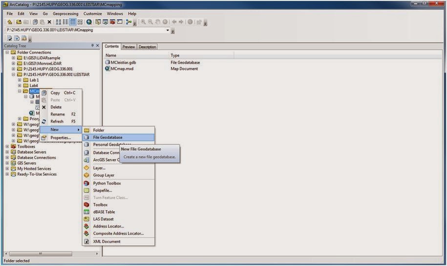
Figure 1 - To create a new file geodatabase, right click in the folder you want your geodatabase to be in, go to new, "File Geodatabase."

The next step is to right click on your newly created File Geodatabase and go to the properties option, like shown in Figure 2.
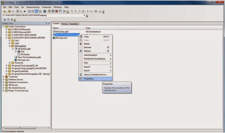
Figure 2 - To get to the domain menu, right click on your File Geodatabase and go to properties.

Near the top of your properties window, click on the "Domains" tab.  In this menu, you can type in whatever field name you are going to be collecting data for in the field.  Make this name short, as this will be referred to later when creating a feature class in your geodatabase.  In the description part of the table, you can explain the domain name further if need be.  Below the initial table is where you can set domain properties.
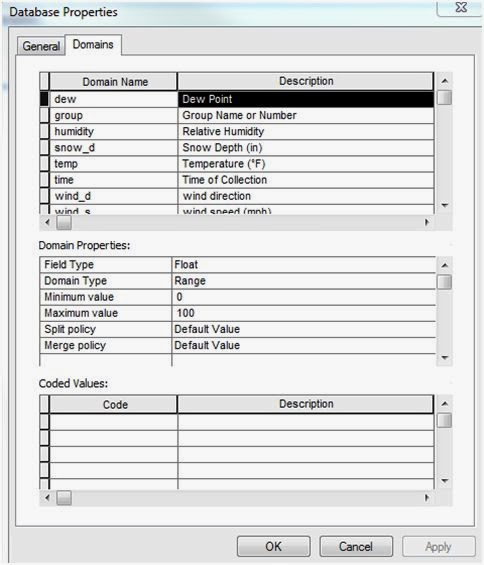
Figure 3 - This figure show domain properties for dew point.


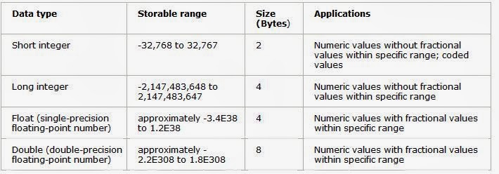
There are a few options when choosing a field type.  Figure 4 shows what the options are and what they mean.  Figure 5 gives a better idea of when to use these different field types.
Figure 4 - This is a figure from ArcGIS Resources that tells what each file type option means.
Figure 5 - This figure shows the extent that the different file types can encompass along with their size and a few applications.

Whenever field work is being conducted, it is a good idea to identify your group name or number as a part of your data.  Since our class is relatively small, we use short integer for groups 1 through 10 (Figure 6).
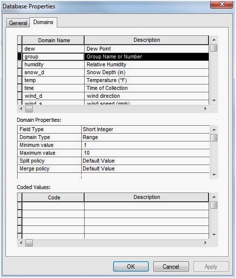
Figure 6 - Domain properties for group name or number.

Since we are setting up this geodatabase to look at a micro-climate map, it is a good idea to include relative humidity in our data.  This can only be a range from 0-100% (Figure 7).
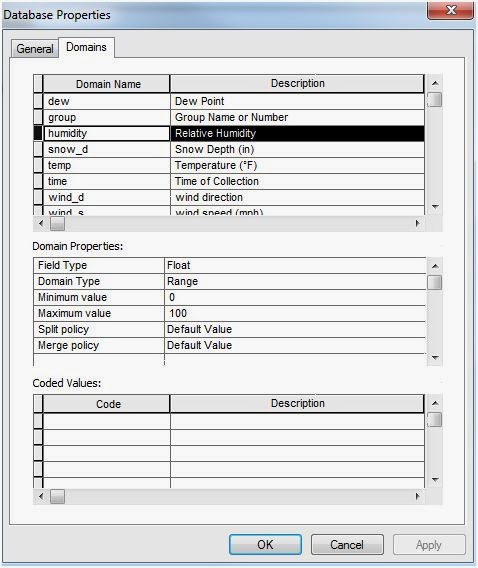
Figure 7 - Domains for relative humidity.

By the time we actually do this exercise, snow depth may not be a factor, but it is an extra attribute that can be added to our geodatabase just in case.  We set this as a float, just so we can be more precise if we decide to measure this in the field (Figure 8).
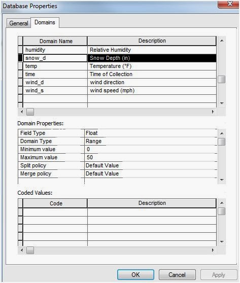
Figure 8 - Domain properties for snow depth.

Temperature is the most important part of the microclimate map.  We set the range from -10 to 100, just because you can never be too sure what the weather is going to be like in Wisconsin (Figure 9).
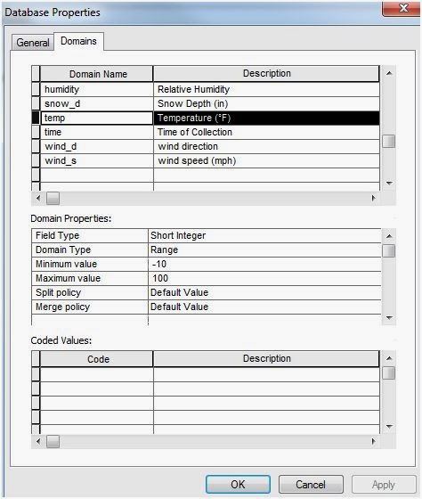
Figure 9 - Domain properties for temperature.

The time is a very important part of the data for the micro-climate exercise because the groups are going to be collaborating all of their data to make one cohesive map.  We will collect this using a military style time, so our range is from 0-2400 (Figure 10).
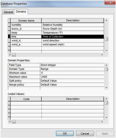
Figure 10 - Domain properties for time of collection.

Wind direction will be measure based on which direction the wind was coming from.  A basic azimuth will be taken for that data, which ranges from 0-360 (Figure 11). 
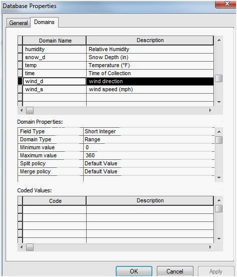
Figure 11 - Domain properties from wind direction.

Wind speed is another important factor when looking at a micro-climate map.  We set a range from 0-60 mph because you cannot have a negative wind direction, and anything higher than 60 would be difficult to even stand in (Figure 12).
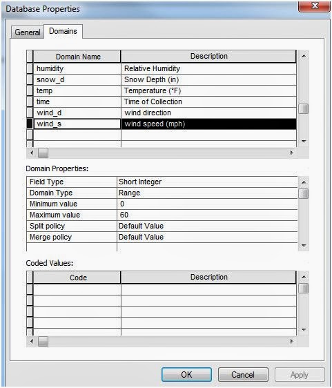
Figure 12 - Domain properties for wind speed.


Now that you have set your domains and domain properties in your new File Geodatabase, you can create a new feature class within that geodatabase.  Figure 13 shows you where to set that up.
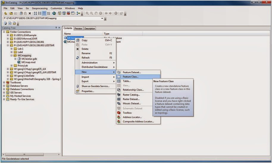
Figure 13 - To get a new feature class, right click on your new File Geodatabase, go to New, then click on Feature Class.


The first screen to appear looks like Figure 14.  This is where you can name your new Feature Class and decided what type of feature your data will be stored as (point, line, polygon, multipoint, multipatch, dimension, or annotation features).  For the micro-climate map, we want our data to be stored as point features.  Use a name that uses your name/username so that you can easily find it later when collaborating data with other students.
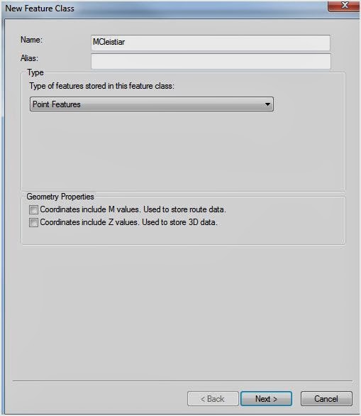
Figure 14 - This is the first screen to come up with creating a new Feature Class.  After making your options look something like this, you can click next.

Next you need to decide what coordinate system your data is going to be projected in.  NAD 83 is usually a good choice (Figure 15), which can be found in the Projected Coordinate Systems, then State Systems.
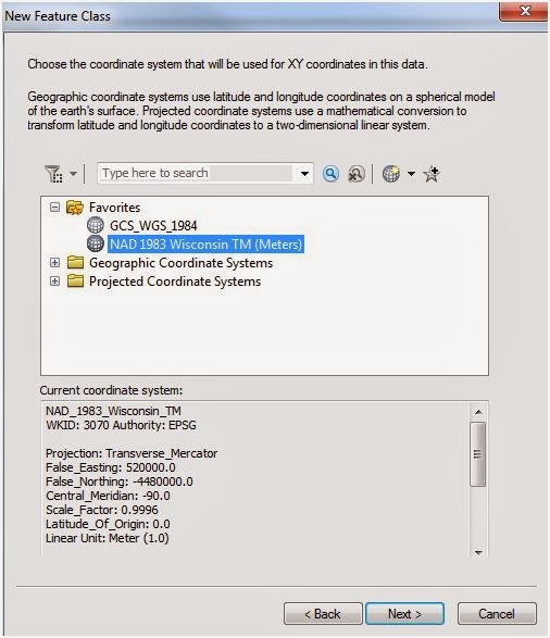
Figure 15 - This coordinate system can be found near the end of the folder named "State Systems" in the Projected Coordinate Systems.

The next two windows can be left as the default options.  The next window is where you can add all the different fields of data that you want to collect in the field.  Figure 16 shows what comes up automatically when this window comes up.
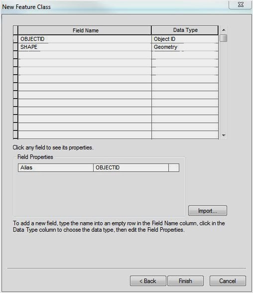
Figure 16 - This is the table to add the fields of data to be collected in the field.

All of the field names in Figure 17 should be added to this window.  This is where you can type in the field name however you want it to show up when you collect the data in the field.  When you click in the cell to the right of the field name you just typed, a drop down list appears of all those field type options that are shown in Figures 4 and 5.  Choose the same data type for that type of data that you set up in your domains.  In field properties in the lower half of the feature class properties window will be a field properties set of options.  In the cell to the right of domain, you should be able to choose the same field name as you have typed in this window.  It will give you all of the options for the data type you have set in your domains before creating a new feature class.
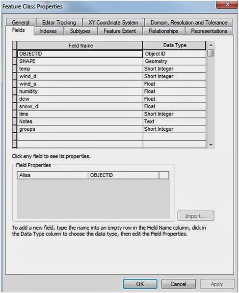
Figure 17 - This shows all the field types that should be included in your feature class.  It is important to add a notes field any time you collect data in the field because you can describe any anomalies in the data here. 

Figure 18 shows just one example of what your field properties should look like.  Temperature is highlighted and I have chosen Short Integer for the Data Type because that is what I had previously decided temperature data would be collected in (which is already set in my file geodatabase domains).  I have a few fields designated with data type as short integer.  When clicking next to domain in the field properties group, temperature, time, wind direction, and wind speed all show up as an option because their domains are all set to short integer.  Make sure you choose the correct field in this step.
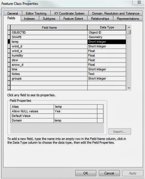
Figure 18 - This figure is showing temperature as an example of what the field properties will look like.  Similar steps need to be taken for all the field names.

Once you click OK, your new feature class will be created.  You can go back in at any time before collecting the data to add, remove, or edit field names, data types, or domains.

Mar 2, 2014

Preparation for Orienteering at the Priory

Introduction

     To do any sort of land navigation, it is great to have top notch technology to tell you where to go.  Unfortunately, no matter how advanced our technology is, it can still have glitches and failures at the most inconvenient times.  For this reason, it is still important to learn how to navigate using traditional methods with a map and a compass.
     On February 24, 2014, we learned a few handy tips on traditional orienteering field methods.  As a class, we went outside figured out what our pace was.  This can help with rough estimates of distances when navigating in the field.  Al Wiberg who is the program director at the Environment Adventure Center (EAC) at the University of Wisconsin Eau Claire also visited our class that day to teach us basics about how to learn a compass out in the field.  We will be going out into the priory in Eau Claire to put these skills to the test once the snow melts.  Before going out into the field though, it is good practice to study maps of the area of interest to look at land features such as topography and vegetation.  Observing these maps in different measurements of latitude and longitude can give the researcher a better idea of the scale of their area.  For this exercise, we are to display the map of the study area in a geographic coordinate system, which will give our coordinates in decimal degrees, and a projected coordinate system of the Universal Transverse Mercator, which will give coordinates in meters.  Data for the study area boundaries were given by Joe Hupy and imagery for the maps was provided by ESRI in ArcMap 10.2.

Methods

Finding your pace

     When conducting field work, it is important to have estimate how far you have traveled even if you do not have high tech field equipment to tell you.  To compensate for the lack of equipment, it is convenient to know what you "pace" is.  One pace is considered two steps, so let's say every time you step on your left foot is considered one pace.  As a class, we measured out 100 meters using a laser range finder (described in better detail with a photo in the previous blog post).  Each student walked that 100 meter distance and counted their own personal pace.  We went through this process twice and took an average of the two pace counts to get a more accurate measure of what our typical pace would be.  My average was 68 paces per 100 meters.  This will be useful when actually going out into the field because now we will have some idea of how far we are travelling to get to each point.  When actually conducting field work, we were advised to over estimate the amount of paces to make up for the differences in terrain.  You are likely to take smaller steps when moving hill.  Also if the study area is wooded, it is possible that you will need to step over or around branches and other obstructions, which will result in a less accurate pace count.

How to use a compass with a map in the field

Figure One - This is type of compass that our class was taught to use during
 Al Wiberg's lesson.  All of the essential parts of the compass are labeled in this
 figure.  To someone who maybe has not used one of these before, it is important
 to note that the dial rotates in both directions (labeled number 5).
     Al Wiberg's lesson on how to use a compass gave students basic background information on how use and read a compass and also how to use in order to navigate in the field.  That way, no matter how much each student knew about how to use a compass, we were all on the same page.  Figure One below shows the type of compass each student was issued for the purpose of this lecture.

     This kind of compass can be used to find an azimuth when you are in the field.  First you must know your current location on a map by analyzing the contour lines and recognizing land features around you and where their locations correspond to on the map.  Once you have your location, choose a point on the map that you need to go.  Lay the compass on the compass flat on the map and connect the two points together with the straight edge of the compass (your current location with the location you are travelling to).  Next, turn the dial (part 5 of Figure One) so that the orienting arrow (part 3 of Figure One) is pointing North on the map.  There are orienting lines (part 8 of Figure One) that need to be parallel with the lines of longitude on your map; this is how you can tell if your orienting arrow is pointing North or not.  The number on the dial that lines up with the direction of travel (part 2 in Figure One) is your bearing.  For example, if that number reads 223 degrees, then your destination is at a 223 degree bearing only from your current location.  Figure Two shows what this process is supposed to look like.


Figure Two - This simple sketch is showing how to find a bearing of a location in respect to your current location.

Preparing the maps in ArcGIS

     Now we know how to use a map and compass in the field, but we still need to prepare our maps before going into the field.  It is very important to some measure of what the topography is doing in your study area, so you know what you are up against.  This is not a huge deal for our study area because the elevation change is not too drastic, but it is still important to research this ahead of time before going out into the field.  I used a 5 meter contour interval on my maps, as it seemed appropriate given the low change in topography.  As a basemap, I used World Imagery provided by ESRI with a translucent DEM overlain on top of that.  The colored DEM gives an idea of where there is similar topography across the map area.
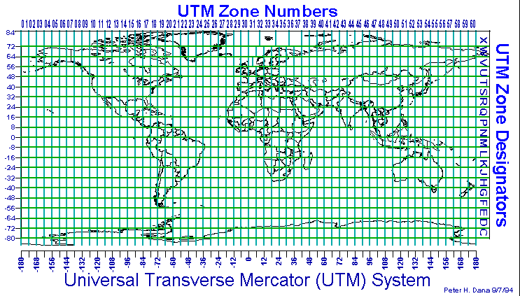
     It is also very important to overlay a grid on the map so that points taken in the field can have a more accurate set of coordinates.  For the priory maps I have produced, I used two different grid systems.  The first kind is a Universal Transverse Mercator grid (Figure Three).  The x-axis is measured on how many meters away that point is from the prime meridian.  The y-axis is measured on how many meters away from the equator.  Figure Three roughly shows how the Earth is broken up into its different UTM zones.  Decimal degrees measures the angle between the very central point within the Earth's core and where the point in question is.  Figure Four does a good job illustrating this point.
Figure Three - This is roughly how the UTM system is broken down.  

Figure Four - This picture shows how latitude and longitude is determined using the decimal degrees system.

     A few steps need to be taken to overlay a grid on your data.When you are in the ArcMap program and all of your data is on your map, make sure you are in the "Layout View" which is being pointed out in Figure Five.
Figure Five - The red arrow is pointing to where the Layout View is in ArcMap.  The other viewing option is the Data View, which is what ArcMap automatically goes to when opening the program.   That is the mode to be in when adding data to your map, but adding a grid system is in the Layout View

Next, right click anywhere in your frame and click on properties.  At the top of the Data Frame Properties window, there is a "Grids" tab on the right side of the window.  One of the first options there is "New Grid" (Figure Six)
Figure Six - This figure is showing what the Grids tab in the Data Frame Properties window looks like.
First, I will show how to get a UTM grid to overly the map.  When the Grids and Graticules Wizard comes up, click the second option for the UTM, which reads "Measured Grid: divides map into a grid of map units."  Figure Seven shows this window with the correct option selected.

Figure Seven - This is the first window of the Grids and Graticules Wizard.  The second option will result in a UTM grid on your map.  When this is selected, click next.

 The next window in the Wizard is where you can set the intervals of both the x and y axis of the grid.  For this project, the both intervals will be set at 50 meters on the x and y axis.  This is seen near the bottom of Figure Eight.

Figure Eight - This shows the next part of the Grid and Graticule Wizard.  With the data that is already in our data frame, the Wizard knows that our units are going to be in meters.

The next two windows in the Wizard deal with how the grid is displayed over the map.  All other defaults were accepted for the priory map.

To get a grid that shows coordinates in decimal degrees, navigate to the same Grid and Graticule Wizard (see Figure Six).  For this new coordinate system, choose the first option in the (Figure Nine).
Figure Nine - This figure shows the proper option selected to give a grid system in decimal degrees.

The next window is where you can set the intervals of your grid system.  Since this system of latitude and longitude will be in degrees, minutes, and seconds, be mindful of the interval you chose.  For this project, I chose an interval of 2 seconds for both the latitude and longitude (Figure Ten).
Figure Ten - This window shows how to set the interval for the decimal degree grid.  
Again, the next two windows in the Grid and Graticule Wizard just deal with formatting preferences.  All other defaults can be accepted for this map.

Results

     Figure Eleven is the resulting map with a UTM grid, while Figure Tweleve uses a decimal degree grid on top of the map.  World imagery from ESRI is used as a basemap.  DEM data is on top of the imagery, but set as 50% transparent so that the imagery can still be seen.  On top of the DEM data is contour data with a 5 meter interval with labels to allow for easier map reading in the field.  The navigation boundary is outlined in yellow to make sure the area of interest is clearly visible against the map.
Figure Eleven - Map of the priory using the UTM grid system.

Figure Twelve - Map of the priory using decimals degrees as a grid system.

Conclusions

     Technology can help make field work a lot easier, but if it fails, it is still important to know how to use traditional methods.  I know have useful maps for the study area that will be easy to read and interpret in the field.  I also now know my pace, which will help me figure out distances when navigating in the field area.  I am eager to take these maps out in the field and put my orienteering lessons to the test.